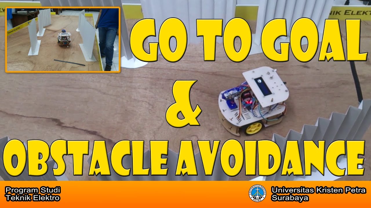
Stability - stability of control system

I want to talk about stability, because as you

probably recall when we did a control

design, first order of business is to

design controllers so that systems don't

blow up. If they blow up, there's nothing

we can do about it. The quad rotors just

fall out of the air. The robots drive off

to infinity. The cars smash into things.

We don't want them to blow up, because the

deciding objectives are almost always

layered in this sense. First order of

business is stability. Then we want to

track whatever reference character or

reference point we have. We also want it

to be robust to parameter uncertainties,

and possibly noise. And then we can wrap

other objectives around it, like when you

want to move as fast, quickly as you can,

or use as little energy when you're

moving, or things like this. But,

regardless of which, stability is always

the first order of business. So let's

start with scalar systems, no inputs. So

only the A matrix now, in this case x dot

is little ax, which means that it's

scalar. Well then the solution x of t is e

to the a, we said t minus t naught x of t

naught. Here I simply picked t naught to

be equal to 0. So this is the solution.

Okay, lets plot what this solution looks

like. If a is positive, then x of t it

starts nicely and then pabaah. Its, its

blowing up as far as I can tell. So if a

is positive this system blows up. Well, if

a is negative, then e to the at, this is a

decaying exponential. So we get x to just

go, , nice down to zero. What happens if a

is zero in between these 2? Well, then you

have e to the zero t, which is 1. So then,

x of t is simply equal to x naught. x

never changes.

So here, it didn't blow up, but it didn't

actually go down to zero. And in fact,

what we have its, its really a sitution

where three possible things can happen you

blow up, you go down to zero, or you stay

put. So let's talk about these three

cases. The first case is what is called

asymptotic, stability. So the system is

asymptotically stable if x goes to zero

For all initial conditions, so this fancy

upside down a, is known as the universal

quantifier. All we need to know is that

when we see and upside down a the way we

pronounce it is for all x nought. So

asymptotic stability means that we go to

zero and almost always what we want to

design our system so that x actually goes

to 0 no matter where we start, that's

asymptotically stability and as you

recall, in the scalar case, a strictly

negative corresponds to asymptotically

stability. And then we have unstability,

instability where the system being

unstable. What that means is there exists

an initial condition, so the flipped e,

and to speak for the existential

quantifier, which we read it as exists. So

it's unstable if there exists so many

extra conditions from which the system

actually blows up. In the scaler case, we

had A positive corresponding to

instability. and then we have something we

call critical stability, which is somehow

in between. The system doesn't blow up.

But it doesn't go to zero either, and in

fact, for the scalar system, this

corresponded, corresponded to the, a equal

to zero case. So if you summarize that, if

you have a scalar system then a positive

means the system is unstable. A negative

means that the system is asymptotically

stable, which is code for saying that the

state goes to zero. And a zero means

critically stable. Okay.

Let use this way of thinking now on the

matrix case. X. is ax, capital A. So this

is now, x is a vector, a is a matrix. What

do we do there? Well, we can't just say.

Oh, a is positive, or a is negative.

Because a is a matrix. It's not positive

or negative. But what we can do is we can

go for the next best thing, which is the

eigenva lues.

And, in fact, almost always, the intuition

you get from a scalar system translates

into the behavior of the eigenvalues of

these matrices. And for those of you who

don't know what eigenvalues are, these are

the special things that are associated

with matrices. So, if I have a matrix A; N

by N, and I multiply it by a vector an N

by 1 vector, if I can write it as the same

vector times a scalar, then what this

means is that the way that A acts on this

vector is basically scaling it. And the

scaling factor is given by lambda. If I

can, if I can find lambda of v to satisfy

this, then what I have is a lambda that is

called an eigenvalue. And it's actually

not a real number. It's typically a

complex number. So it's a, a slightly more

general object than just a real number,

but that's an eigenvalue. And v is known

as an eigenvector. And eigenvalues and

eigenvectors are really these fundamental

objects in, in when you're dealing with

matrices and when you want to understand

how they behave. And, whenever you think

scalar first, you can almost always

translate it into what do the eigenvalues,

eigenvalues do for your systems. And, the

eigenvalues actually would tell you how

the matrix a acts in the directions of eh

eigenvectors. So, you can almost think of

them as scalar systems in the directions

of the different eigenvectors. And, you

know, sometimes you may want to compute

eigenvalues. I don't.

So, if you use MATLAB. You would just

write, eig(A), and out pops the

eigenvalues. whatever software you, your

comfortable with, you want to use C, or

Python, or whatever, there is almost

always a library that allows you to

compute eigenvalues. And, the command is

typically something like eig(A).

So, this would give you what eigenvalues

are, given a particular matrix. Okay.

Let's see what this actually means. Let's

take a simple example here. Here's my a

system. 1, 0, o minus 1. if you take eig a

of this. you get 1 eigenvalue being 1. And

the other eigenvalue being negative 1. And

the correspo nding eigenvectors are 1, 0,

and 0, 1. Okay.

What does this mean? It actually means the

following. So let's say that this is x1,

and this is x2. Okay.

V2 was 0, 1. So this was this direction.

So here is what, v2 is. This is the

direction in which v2 is pointing. Well,

the eigenvalue there is negative 1, which

means that, if you recall the scalar

system, when a was negative, we had

stability. So if I start here, my

trajectory is going to pull me down to

zero. Nice and stable, and in fact, if I

start here, it's going to pull me up to

zero, nice and stable. Right.

So, if I'm starting. on the x2 axis, my

system is well behaved. If I start on the

x1 axis, I have lambda 1 being positive,

which corresponds to little a being

positive in the scalar case, which means

that the system actually blows up. So,

here, the system goes off to infinity.

And, in fact, if I start here, my x2

component is going to shrink but my x1

component is going to go off to infinity.

So what I have is this is what the system

actually looks like. So the eigen vectors

in this case will tell me what happens

along different dimensions of, of the

system. So after all of this, if I have x

dot as big AX, and I can find a solution,

then the system is asymptotically stable,

if and only if, for the scalar case, we

had that little a had to be negative. What

we need in the matrix case is that the

real part, remember that Lambda are

complex, the real part of Lambda is

strictly negative for all eigenvalues to

a. For all, this is what asymptotic

stability means for linear systems.

Unstable means that there is one or more,

but one single bad eigenvalue spoils the

whole bunch. So a single eigenvalue that

has positive real part. This is an, a

sufficient condition for instability. And

we have critical stability only if so this

is a, a necessary condition that says the

real part has to be less than or equal to

0 for all igon values. But where we are

going to be spending our time is Typically

up here in the asymptotically stabl e

domain, because what we want to do, is we

want to design our system or our

controllers in such a way that the closed

loop system is asymptotically stable. So

we're going to somehow make the eigen

values have negative real part That's

going to be one of the design objectives

that we're interested in. And I want to

point out something about critical

stability that if one eigenvalue is 0 and

the rest of the eigenvalues have negative

real part, or if you have two purely

imaginary eigenvalues So they have no real

part, and the rest have negative real

part, then you have critical stability.

and we will actually see that a little bit

later on, but the thing that I really want

to take, you to take with you based on

this slide, is, you look at the a matrix,

you compute the eigenvalues. If the real

part of the eigenvalues are all negative

You're free and clear, the system is

asymptotically stable. If one or more

eigenvalues have positive real part, you

toast, your system blows up. That is bad.

So, let's end with a tale of two pendula.

Here is the normal pendula, well if you

compute the of this, you get this matrix.

And the eigenvalues are j and negative j.

Well, I don't know if you remember, but on

the previous slide, there was a bullet

that said if you have 2 purely imaginary

eigenvalues, which we have here. We have 2

purely imaginary eigenvalues and then no

more, then we have critical stability.

What this actually means is that, this

pendulum, clearly, there is no friction or

grav-, or damping here. It's just going to

oscillate forever. It's not going to blow

up. And it's, , excuse me. And it's not

going to go down to zero. It's just going

to keep oscillating forever and ever. It's

critically stable system.

Now, let's look at the inverted pendulum

where I'm moving the base, but in that

case, a is 0110. We already know, this

things is going to fall over. Right? So,

if you compute the Eigen values you get

one Eigen value to be equal to negative 1

and 1 to be positive 1, which means that,

we have one Rothton eigenvalue. This

eigenvalue that's going to spoil the

system. So this in an unstable system. So

now that we understand that eigenvalues

really matter, and they really influence

the behavior of the system, let's see, ,

excuse me, how we can use this to our

advantage when we do control design.

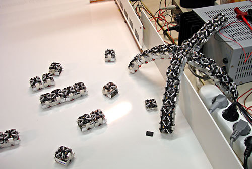
Swarm Robotics - Swarm Robotics projects - Control of Mobile Robots

Swarm Robotics

So, in the previous lecture, we saw that

eigenvalues play a fundamentally important

role when you want to understand stability

properties of linear systems. We saw that

if all eigenvalues have strictly negative

real part, the systems are asymptotically

stable. If one eigenvalue is positive,

then we have positive real part. Then,

we're screwed and the system blows up.

Now, today, I'm going to use some of these

ideas to solve a fundamental problem in

swarm robotics. And this is known as the

Rendezvous Problem. And, in fact, what it

is, is you have a collection of mobile

robots that can only measure the relative

displacements of their neighbors. Meaning,

they don't know where they are, but they

know where they are relative to the

neighbors. So here, here we have agent i,

and it can measure xi minus xj, which is

actually this vector. So, it knows where

agent j is relative to it. And this is

typically what you get when you have an

censor skirt, right? Because, you can see

agents that are within a certain distance

od you. And, as we saw, you know, where

they are relative to you. If you don't

have global positioning information, you

don't know where you are so there's no way

you're going to know, globally, where this

thing is, but you know where your

neighbors are locally. And the Rendezvous

Problem is the problem where having all

the agents meet at the same position. You

don't want to specify in advance where

they going to meet because since they

don't know where they are, they don't know

where they going to meet. They can say,

oh, we're going to meet in, at the origin.

But I don't know where the origin is. Is

it in, in Atlanta, Georgia? Or is it in

Belgium, or is it India? What do I know,

right? So, the point is, we're going to

meet somewhere, but we don't know where.

Okay.

So, we have actually solved this problem

before. We sold it for the 2 robot case,

where we had 2 robots. and we could

control the velocities right away. What we

did is we simply had the agents aim

towards each other. So, u1 was x2 minus

x1. And u2 was x1 minus x2. This simply

means that they're aiming towards each

other. Well, if we do that, we can

actually write down the following the

following system. This is the closed loop

system now, where we have picked that

controller. So, x dot is this matrix times

x. Okay, let's see if this works now.

Well, how do we do that? Well, we check

the eigenvalues of the A matrix to see

what's going on. Alright. Here is my A

matrix, type eig in MATLAB or whatever

software you're using, and you get that

lambda 1 is 0, lambda 2 is negative 2.

Okay, this is a little annoying, right?

Because we said asymptotic stability means

that both eigenvalues need negative real

part, this doesn't have that. But

asymptotically stable, so asymptotic

stability also means that the state goes

to the origin and, like we said, we don't

know where the origin is, so why should we

expect that? We should not expect it. We

also know that one positive eigenvalue or

eigenvalue with positive real part makes a

system go unstable. We don't have that

either. In fact, what we have is this

in-between case that we called critical

stability. We have one 0 eigenvalue and

the remaining eigenvalues have negative

real part. So, this is critically stable.

And, in fact, here is a fact that I'm not

going to show but this is a very useful

fact. So, that if you have one eigenvalue

be zero and all the others have negative

real part, then in, in a certain sense,

you're acting like asymptotic stability.

Meaning, you go, in this case, not to zero

but you go into a special space called the

null space of A. And the null space of A

is given by the set of all x, so such that

when you multiply A by x, you get zero

out. That's where your going to end up.

So, your going to end up inside this thing

called the null space of A, in this case,

because you have one 0 eigenvalue and all

others having strictly negative real part.

And if you type null(A) in MATLAB, you

find that the null space for this

particular A is given by x is equal to

alpha, alpha where alpha is any real

number and why is that? Well, if I take

negative 1, 1, 1, negative 1, this is my A

matrix, and I multiply this by alpha,

alpha, what do I get? Well, ll' get minus

alpha plus alpha here, and then I get plus

alpha minus alpha there, which is clearly

equal to 0. So, this is the null space.

Okay, what does this mean for me? Well, it

means that x is, x1 is going to go to

alpha and x2 is going to go to alpha. x1

goes to alpha, x2 goes to alpha, which

means that x1 minus x2 goes to 0 because

they go to the same thing. Which means,

that we have, ta-da, achieved rendevous.

They end up on top of each other. In fact,

they end, end up at alpha. We don't know

what alpha is but We know that they end up

there. Okay.

Now, if you have more than two agents, we

simply do the same thing. In this case, we

aim towards what's called the centroid of

the neighbors. And, in fact, if we write

this down, we write down the same thing

for more than one agent, we get that x dot

i, before it was just xj minus xi, there

were 2 agents. Now, I'm summing over all

of agents i's neighbors. That is doing the

same thing if you have more than one

agent. And, in fact, if you do that and

you stack all the x's together then you

can write this as x. is negative lx. And

this is just some bookkeeping. And the

interesting thing here, here is that l it,

it's known as the Laplacian of the

underlying graph. Meaning, who can talk to

whom. that's not so important. The

important thing though is that we know a

lot about this matrix L and, again, and

it's called the graph Laplacian. And the

fact is that if the undergrinding,

underlying graph is connected, then L has

one 0 eigenvalue, and the rest of the

eigenvalues are positive. But look here,

we have negative L here, which means that

negative L is one 0 eigenvalue and the

rest of the eigenvalues are negative.

That means that this system here, the

general multiagent system here is actually

critically stable. And we know that it

goes int o the null space of L. And it

turns out, and this is a fact from

something called algebraic graph theory.

We don't need to worry too much about it.

We just know that clever graph

theoreticians have figured out that the

null space to L, if the graph is connected

which means that there is some path with,

through this network between any two

agents is given by not alpha, alpha but

alpha, alpha, alpha, alpha, alpha, a bunch

of alphas. So, just like before, if I have

this thing and, in fact, it doesn't have

to be scalar agents, what I do have is

that all the agents go to the same alpha

or in other words, the difference between

the agents will actually disappear. And

when we did this, we design a controller.

We actually designed this thing here. And

this thing is so useful that it actually

has its own name. It's known as the

consensus equation because it makes agents

agree. In this case, they were agreeing on

position. But this equation actually will

solve the rendezvous problem because of

the fact that the corresponding system

matrix you get is negative L at the right

eigenvalues which means that the system is

critically stable so we can solve

rendezvous in the multirobot case. And

again, you've seen this video. Now, you

know what it was I was running to generate

this video. In fact, you can go beyond

rendezvous So, here is actually a course

that I'm teaching at Georgia Tech, where

you want to do a bunch of different

things. And again, all I'm doing is really

the rendezvous equation with a bunch of

weights on top of it. And we're going to

learn how to do this. I just want to show

you this video, because I think it's quite

spectacular. You have robots that have to

navigate an environment. They're running

these, basically the conses equation and

they have to avoid slamming into

obstacles, so I should point out that this

was the final project, project in this

course, it's called network control

systems. And I just wanted to show you

that you can take this very simple

algorithm that we just dev eloped, make

some minor tweaks to it, which we're going

to learn how to do, to solve rather

complicated, multiagent robotics problems.

So here, the robots have to split into

different subgroups and avoid things, they

have to get information, they have to

discover missing agents and so forth. And

we will learn how to do all of that in

this course. Now, having said that, talk

is cheap, right? And simulation is maybe

not cheap, but let's do it for real. In

this case, we're going to have two Khepera

mobile robots, and what we're going to do

is we're going to use the same PID

go-to-go controllers and we're going to

let the consensus equation flop down

intermediary goal points. And what we're

going to do is we're going to keep track

of our position using odometry, meaning

our, our real encoders. And what the

robots are going to do, is they're

actually going to tell each other where

they are rather than sense where they are

because we haven't talked yet about how

the design sensing links. So, what we're

doing is we're faking the sensing and

telling, they're telling each other where

they are. And they're using a PID

regulator to go in the direction that the

consensus equation is telling them to go

in. And now, let's switch to the actual

robots running and solving the rendezvous

problem. So, now that we have designed a

closed looped controller for achieving

rendezvous we're going to deploy it on our

old friends, to Khepera mobile robots. so,

what we will see now are these two robots

actually executing this algorithm. and we

will be using the same go to goal

controller as we designed earlier to

achieve this. And, as always, I have J P..

De la Croix here to conduct the affairs

and practically, we're going to see two

robots crashing into each other which is

exciting in its own right. But

intellectually, what we're going to see,

is the state of the system asymptotically

driving into the null space of our new A

matrix. And the reason for that is, as

we've seen this matrix has 0, 0

eigenvalue, which means that the system is

critically stable and the states approach

the null space. So, J.P., without further

ado, let's see a robotic crash. So, we see

they're immediately turning towards each

other and . Pretty exciting stuff, if I

may say so myself.

Obstacle Avoidance - obstacle avoidance algorithm - Control of Mobile Robots

So now we feel pretty confident abut our

ability to design controllers that take a

robot to a goal location. In fact we've

seen it in design, we've seen it in

simulation, and we've even seen it in real

life. But we have not discussed the issue

of. Well what if the robot needs to do

something slightly more elaborate than

just get to the point for instance you

typically don't want to hit things on the

way over there so the one behavior that I

want to talk a little bit about is

obstacle avoidance because goal to goal

and obstacle avoidance are really the

dynamic duo of mobile robatics. ,, . We're

going to do more things, of course. But

underneath the hood, there will always be

a goal to goal, and an obstacle avoidance

behavior. And let's think a little bit

about how one should avoid driving into

obstacles. Because going to goal location

was not. Particularly complicated.

Well, we can clearly use the same idea as

we did in go-to-goal by defining a desired

heading, and then simply, you know, steer

in that direction. So, let's say that we

have the following. The robot, well, it's

the blue ball. And then we have this

little red. C, which is the obstacle,

located at xo yo. And the reason that we

know the location of this is because the,

the disc obstraction we talked about, when

we talked about the sensors. Okay, if this

is a goal, we would steer towards it. That

much is clear, now, the question is If it

is an obstacle which direction should we

steer it, when it's not as clear. I mean,

here is a direction we can go in. You

know, let's run away from the obstacle.

But that's a little overly cautious I

think. At least sometimes, if I'm not even

on m way towards the, The red thing. Why

do all of a sudden I have to insist on

going the opposite direction? So. This is

one direction which we can go in, but it

seems a little, how should I put it. It

seems a little skittish, or paranoid. We

should be able to be a little bit more.

Clever, maybe like this. So if we're going

in this general direction, then we should

maybe go perpendicular to the, the

direction to the obstacle. That's one way

in which we could be thinking but there

are other choices we could make. Let's say

that we have a goal. Again, we're not just

avoiding obstacles, we're actually trying

to go somewhere. This obstacle The red

obstacle we see here. Well, it doesn't

seem to matter if I'm going towards the

goal, what do I care about that obstacle.

So, hey we could just ignore it. That's

one direction we could go in. Or we could

somehow combine the direction to the goal

with some way of avoiding an obstacle. So,

we could kind of move away from the

obstacle while somewhat getting towards

it. To goal.

The point here is that there is no obvious

correct answer, going to goal its clear

which direction we want to go in. When

we're avoiding an obstacle its not as

clear, its not obvi, obviously have to go

in this direction and we have choices and

some how some choices are better than

others. So lets, lets look at some of

these choices that we have a little bit.

Okay.

So we have the robot in blue, we have the

obstacle in red. And we have the goal in

yellow. This was choice one. Pi 1 is, I'm

going to call it Pi obst plus Pi. So Pi

obst is this angle, right? So, here is phi

obst. And in fact, Pi obst is we can write

it as arc tangent y obst minus y over x

obst minus x. So this is some way in which

we compute the angle to the obstacle and

then we can say well Pi 1 suggestion one

which is the. The super paranoid robot

who's avoiding obstacles at all cost, it's

adding Pi to the mix. And by the way why

am I adding Pi, and not subtracting Pi?

All right, so, here's the, the, the angle

I want to go to the, this is phi obst.

And, what I'm doing no is adding Pi.

Right, so, this is , well the point is

that it actually doesn't matter if you add

Pi, or subtract Pi, because by now we know

that angles are slightly scary objects.

And, we always take something like r

tangents too, to ensure that we stay

within minus Pi and Pi. Adding Pi or

subtrac ting Pi as long as we take. Some

safety measures, it doesn't matter. So, we

can do the same thing. It doesn't matter

which one we choose. But, that's one way.

Now, this direction is pure in the sense

that I don't care where the goal is. I am

just going to move away from the obstacle

as much as I can. So, I'm going to call

this pure avoidance. No notion of where

I'm supposed to be going. Well, we had

another choice, right? We said, what if we

go perpendicularly to this direction?

Well, so Pi 2 is Pi obstacle plus minus

Pi. Well, what does that mean? It means

that if I do minus Pi over 2, I go in this

direction. If I do plus Pi over 2, I go in

that direction. And there, here it

actually matters if I do plus or minus.

And the question is, which one should we

choose? Well, typically that depends on

where the goal is. So we should pick in

this case minus Pi over 2 because that

moves us closer to the goal, while plus Pi

over 2 moves us further away from the

goal. And the punchline here is really

that this is not a pure strategy, because

we need to know where the goal is.

Instead, what we're doing is we're

actually, I'm calling it blended in, in,

in the sense that we're taking the

direction to the goal into account when we

are figuring out in which direction we

should be going. So it's not a pure

obstacle avoidance. If I just ask you to

avoid an obstacle, you say I can't,

because it needs to know where the goal

is. In that sense, it's not pure. So,

that's one choice. Well, remember this

one? We said, you know what? This obstacle

is no big deal to us, we are just simply

going to go in the direction of the goal.

Well, this is pure goal to goal. We're

just running one behavior. goal to goal,

we don't care about the obstacle. And

what's more interesting is this choice, Fi

4 which is really a combination of the

direction to the goal and the direction to

the obstacle. And the interesting thing

here is that this is clearly a blended

mechanism, somehow we combining go to

goal, type oyds with obstacl e avoidance

of ideas and the punch line here is that

there are really two fundamentally

different ways of combining, avoiding

slimming interstuff and getting to goal

points and these ways of combining things

is called an arbitration Mechanism so we

saw typically in this case two

fundamentally different arbitration

mechanisms one is the winner takes all

approach which is a hard switch when we're

just going straight away from the obstacle

right so here was the obstacle here was

the robot with the robot was going there

we're doing just avoid obstacles. Or, if

the goal was here, right? And we're going

straight to the goal, we're doing just go

to goal. So, these would be two examples

of hard switches. Now, the two other

examples we saw were blended behaviors.

One was, you're combining somehow, the

angle to the goal and the angle to the

obstacle to produce a new desired angle.

and the first blended behavior we saw was

one where we're kind of moving

perpendicularly to the obstacle, but we're

doing it in such a way that we're getting

closer to the goal. And these are two

valid ways of designing arbitration

mechanisms. And in fact, we are going to

have to get systematic and careful about

how to do it. And I should point out that

both Approaches have merit. Now the nice

thing about the winner takes all is that

if go to goal is only going to goal, then

I can analyze that. If obstacle avoidance

is only avoiding obstacles then I can

analyze that, which means that from an

analysis point of view it's easier to deal

with hard switches. However, it's not

necessarily the case that from a

performance point of view hard switches

are to be preferred. Because, it seems

like as I'm walking around I'm kind of

keeping an eye on where I'm going while

not slamming into things. So I'm not

either going towards something or avoiding

slamming into things. So it seems like

performance wise, blending or smoothing

the two behaviors makes a lot of sense.

However, from an analysis point of view

it's harder. So, the question is ho w do

you design your system in such a way that

you can have your cake and eat it meaning

you can analyze what's going on and you

still have good performance. So, we are

going to have to bite this bullet head on,

and in fact we would be very systematic.

And what we have done in this module,

module two is simply introduce mobile

robots. We've looked at some basic models.

We looked at some basic ways in which

we're getting information about the world.

And we designed some basic behaviors, but

to be honest, we haven't been particularly

careful about what we did. Module one, we

were also not particularly careful, but

there the focus was on control theory. So

mobile, mo, , module three is enough chit

chat. Let actually start this course in a

more systematic and formal matter. So,

we're going to return to module one. In

module three and then we're going to

return to module two. And we're going to

see, can we do what we just did, did in a

rather heuristic and ad hoc manner in a

systematic and more formal way. And the

way to do it is to go to the wonderful

abstraction that is linear systems theory.

So, that is the focus of the next module.

Go to Goal - Control of Mobile Robots

So now that we have established that we

need a goal to goal behavior, and possibly

an avoid obstacle behavior in order to go

between points a and b. and we have

figured out that if we have a differential

drive robot that we can model as a

unicycle. With constant velocity v not.

Then, what we can really control is the,

the heading. And the way we control it is

phi dot is equal to omega. Now, let's

define the error, error equals to phi

desire minus phi. So the desired heading

minus the heading we're in. And then we

could use the PID controller, acting on,

e. And we should remember that we may not

want to act directly on e because it's an

angle, so this little trick with arc

tangents 2 would allow us to ensure that e

stays within minus pi and pi. Okay, let's

use this to actually build a behavior that

takes us to a goal. So, the question then

is, the only unknown here, which is what's

phi desired? Well, say we, we're located

at x and y, we know where the goal is, x

goal and y goal. And, the way we know it

is, either because of the sensor skirt

disc extraction we talked about, or some

other way of knowing the goal location.

Well, it's not very hard to compute what's

the desired angle is. It's simply y goal

minus y divided by x goal minus x, and

then r tangent of that. So phi desired in

this case, of course, is this angle here.

So that's given by this arc tangent

formula. So now all we do is we plug it in

to get the error, then we plug the error

in to get the controller and then we hook

the controller in to get the update on, on

the heading. Okay, so without further ado,

let's do it. Okay, here's my first.

attempt, look at this we're getting there,

what? Alright what just happened here?

This was attempt 1 and well, the robot

started out, started out looking in the

wrong direction and then it was starting

to turn nicely, maybe not enough but, and

then something happened, and it seem to

happen roughly when the angle here was

close to minus pi over 2, but in fact this

is exactly what happened. The problem here

is that I forgot that I was dealing with

angles So the issue is, da, da, da, da,

angles. As we talked about, let's not plug

in angles right away. Let's always make

sure that they are within -pi and pi. And

by the way, only in this case was just k

times the error. So it was a pure p

regulator. No i and no t part. But this is

what happens. Even if you do a nice design

and you forget that you're dealing with

angles instead of other entities. So.

Let's go to attempt two. The same

controller. Now I'm putting omega equal to

within quotations here. This simply means

that it's not exactly this, because I'm

doing the arc tangent 2 on this. And,

let's see what the robot is doing. It's

spiraling around the starry air a little

bit. Eh, not, not that great, I must say.

So what seems to be the matter? Well, the

problem is the following. I'm driving the

car at a constant speed, V naught.

And then I'm turning based on this

equation up here. And it doesn't seem like

I'm turning fast enough. You know, if I'm

going really fast, then I need to turn a

lot to, to, actually get to where I want.

So the problem is simply that I'm not

turning quickly enough. Or maybe I should

slow down when I get closer to an

obstacle. And, in truth, if you're

controlling v and omega at the same time,

you need to be a little bit more, you need

to be cle-, more smart in your control

design than just a PID regulator on the,

the heading error. But, since this is what

we're doing right now, simply what we

should observe is the gain is not high

enough. K is not high enough to steer us

towards where we would like to go. So,

let's do the same thing. But let's make k

bigger. So this is attempt 3. We're doing

the same thing. We have k big. And again,

we have the quotations there, because it's

not exactly this we're doing. What we're

really doing is this arc tan 2 trick on

the, the error on the angles, to make sure

that we get something between -pi and pi.

And, this is just right. This was a

successful control design and in fact,

pure p part, and I don't know if you

remember this video that I showed you that

showed how the metric drift was happening.

It was this video. Well, let's look at it

again. >> Go!

>> And, this time I have the volume up,

because it's really exciting! This is a

competition, and what these robots are

doing is exactly what we just saw.

Obstacle, no, goal to goal using a P

regulator, and this is a competition of

the P games. And, in this case, one robot

did well, and the other was forced out of

bounds. But, this was exactly the

controller. that was running on this kind

of robot.

Okay.

Behavior Based Robotics - Control of Mobile Robots

the world is fundementally dynamic and changing and

unknown to the robot, so it does not make

sense to overplan and think very hardly

about how do you act optimally given these

assumptions about what the world looks

like. That may make sense if your

designing controllers for an industrial

robot at a manufacturing plant where the

robot is going to repeat the same. Motion

over and over and over again. You're going

to do spot welding, and you're going to

produce the same motion 10,000 times in a

single day. Then you'll overplan. Then

you'll make sure that you're optimal. But

if a robot is out exploring an area where

it doesn't know exactly what's going on,

you don't want to spend all your

computational money on Finding the best

possible way to move. Because, it's not

actually going to be best. Because the

world is not what you thought it was. So

the key idea to overcome this that's quite

standard in robotics, is to simply develop

a library of useful controllers. So these

are controllers that do different things.

Like going to landmarks, avoiding

obstacles. We saw one that tried to make

robots drive through center of gravity of

their neighbors. Basically, we can have a

library of these useful controllers,

behaviors if you will, and then we switch

among these behaviors in response to what

the environment throws at us. If all of a

sudden an obstacle appears, then we avoid

it. Then if we see a power outlet and

we're low on battery then we go and

recharge. So we're switching to different

controllers in response to what is going

on. So what I would like to do is to start

designing some Behaviors just to see how

what we learned in module one, a little

bit about control design can be used to

build some behaviors. So let's assume we

have our differential-drive mobile robot.

And to make matters a little easier up

front, we're going to assume that the

velocity. The speed is, is constant. So v

not. We're not going to change how quickly

the robot is moving. So what we can change

i s how we're steering. So you're

basically sitting in a car on cruise

control, where the velocities are

changing, and you steer it. That's your

job. And the question is, how should you

actually. >> Steer the robot around. So,

this is the equation then, that's

governing how the input Omega, it's the

state that we're interested in, in this

case pi, which is the heading of the

robot. So, pi dot is equal to Omega. Okay,

so, let's say that we have our. >> Yellow

triangle robot, it's a unicycle or

differential-drive robot. It's headed in

direction five, so this is the direction

it's in. And, for some reason, we have

figured out that we want to go in this

direction, five desired or 5 sum D. Maybe

there is something interesting over here,

that were interested in. So, we want to

drive in this direction. Well, how should

we actually do this? Well, pi dot is equal

to Omega. So, our job clearly is that of

figuring out what Omega is equal to, which

is the control input. Alright, so, how do

we do that? Well, you know what? We have a

reference, pi desired. Well, in module

one. we called references r. Right? We

have an error, meaning, that compares the

reference pi desired to what the system is

doing. In this case, pi. So it's comparing

the headings. So we have an error, we have

a reference. You know what? We have a

dynamics. pi dot is equal to Omega. So we

have everything we had towards the end of

module one. So we even know how to design

controllers for that. How should we do

that? Well, we saw PID, right? That's the

only controller we've actually seen. So,

why don't we try a PID regulator? That

seems like a perfectly useful way of

building a controller. So, you know what,

Omega is Kp times e, where Kp was the

proportional gain. So this response to

what the error is right now. You make Kp

large it responds quicker but you may

induce oscillations, then you have the

integral of the error. So you take the e

of tau, the tau times k sub i, which is

the integral gain. And this thing, this

integral, has the nice property that it's

integrating up all these tiny little

tracking errors that we may have, and

after a while this integral becomes large

enough that it pushes the system Up to no

tracking errors, that's a very good

feature of the, the interval. Even though

as we saw we need to be aware of the fact

that a big KI can actually also induce

oscillations and then we could have a d

terms. A KD times e dot and that where KD

is the, the gain for derivative part. This

makes the system. Very responsive but can

become a little bit oversensitive to

noise. So will this work? No it won't. And

I will now tell you why. In this case

we're dealing with angles. And angles are.

Rather peculiar beasts. Let's say that phi

desired a 0 radiance. And my actual

heading now, phi is 100 radiance. Then the

error is minus 100 radiance. Which means

that this is a really, really large error.

So Omega is going to be ginormous. But,

that doesn't seem right. Because 100 pi

radius is the same as zero radius, right?

So, the error should actually be zero, so

we should not be niave when we're dealing

with angles. And, in fact this is

something we should be aware of. Is angles

are rather peculiar beasts. And we need to

be, be dealing with them. And there are

famous robotic crashes that have been

caused by this. When the robot starts

spinning like crazy. Even though it

shouldn't. But it's doing it because it

thinks it's 200 pi off instead of zero

radius off. So what do we do about it?

Well the solution is to ensure that the

error is always between minus pi and pi.

So minus 100 pi, well that's the same

thing as zero. So we need to ensure that

whatever we're doing is we're staying

within minus pi and pi. And there is a

really easy way of doing that. We can use

a function, arc tangents two. Any language

there is a library with and it operates in

the same way. It's a way of producing

angles between minus pi and pi. C plus,

plus has it, Java has it, MATLAB has it,

whatever you, Python has it. So you c an

always do this and how do you do that?

Well you take the angle that's now

1,000,000 pi right and You take sine of it

comma cosine of it. So this is the same as

saying that we're really doing arc tan. So

I'm going to write this as tan inverse

sine e over cosine e. But arc tan or tan

inverse. Doesn't, it's not clear what that

always returns but arc tan 2, where you

have a coma in it, you always get

something that's within minus Pi and Pi.

So here's what you need to do, whenever

you're dealing with angles and you're

acting on them, it's not a bad idea to

wrap one of these arc tan two lines around

it to ensure That you are indeed having

values that aren't crazy. So, with a

little caveate that we're going to use e

prime instead of e, the PID regulator will

work like a charm. Okay, so here is an

example problem. We've already seen this

picture. this is the problem of driving

the robot, which is the little blue ball,

to. The goal, which is the sun,

apparently, and lets see if we can use

this PID control design on Omega to design

controllers that take us to the sun, or to

the goal. and since we're dealing with

obstacles and we're dealing with goal

locations, and we're also talking about

behaviors. at the minmum we really need

two behaviors. Goal to goal, and avoid

obstacles. So what we're going to do over

the next couple of lectures, is develop

these behaviors, and then deploy them on a

robot and see if there any good or not.

Sensors | Control of Mobile Robots

We have a model of a robot, we know how

the robot can get position information, in

this case we used the wheel encoders but

there are other ways we talked about

compasses and accele accelerometers but

the robot also needs to know what the

world around. It looks like. And for that

you need sensors. And we are not going to

be spending too much time modeling

different kinds of sensors, and see what

is the difference between an infrared and

an ultrasonic range sensor. Instead.

We're going to come up with an abstraction

that captures what a lot of different

sensing modalities can do. And, it's going

to be based on what's called the, the

range sensor skirt. This is the standard

sensor suite in a lot, on a lot of robots.

And, it's basically a. Collection of

sensors that are. The collection that is,

gathered around the robot. That measures

distances in different directions. So,

infra red skirts, ultrasound. LIDAR, which

are laser scanners. These are all examples

of these range sensors. They're going to

show up a lot. Now there are other

standard external sensors of course,

vision, or tactile sensors, we have

bumpers or other ways of physically

interacting with the world or "GPS" or I'm

putting them in quotation because there

are other ways of faking GPS. For

instance, in my lab I'm using a motioning,

or motion captioning system to pretend

that I have GPS. But what we're going to

do, mainly. It's assumed that we have this

kind of setup. Where a skirt around the

robot that can measure distances to, to

other to things in the environment. And in

fact, here is the Chipera It's a

simulation of the Chipera. And the Chipera

in this case, has a number of infrared

sensors. And Well you see the cones, you

have blue and red cones, and then you have

red rectangles. The red rectangles are

obstacles and what we're going to be able

to do is measure the direction and

distance to obstacles. So this is what

type of information we're going to get out

of these range-sensor skirts. over here on

the right you see two pictures of the

sensing modalities that we had on The

self-driving car that was developed at

Georgia Tech. And we have laser scanners

and radar and vision. but the point is the

skirt doesn't always have to be uniform or

even homogeneous across the sensors. Here

we have a skirt that is heterogeneous

across different sensing modalities. But,

roughly you have the same kind of

abstraction for a car like this, as well

as for. Hey, Chipera, little mobile

differential drive, robot. Okay, so,

that's fine, but we don't actually want to

worry about particular sensors. We need to

come up with an abstraction of this,

sensor skirt, that, that makes sense, that

we can reason about when we design our

controller. So, what we're going to do is,

we're going to do some, or perform what's

called a disk abstract. Abstraction.

So here's the robot, sitting here in the

middle. around it are sensors. And in

fact, if you look at this picture here,

here are little infrared sensors. And in

fact, here are ultrasonic sensors.You see

that scattered around this robot are. It's

a skirt of range censors. We're, they

typically have an effective range, and

we're going to extract that and say there

is a disk around the robot, of a certain

radius, where the robot can see what's

going on, right, so this is this, this

pinkish disk around the robot and it can

detect obstacles that are. Around it.

So the two red symbols there are the

obstacles. What we can do is we can figure

out how far away are the two obstacles.

So, D1 is the distance to obstacle one,

which is this guy. And this is obstacle

two, well, okay. join with ratts of ensure

and Pi one is the angle to that obstacle,

similarly d2 is the distance to obstacle

2. Phi 2 is the angle to obstacle two. One

thing to keep in mind though is that robot

has its own coordinate system in the sense

that this, if this is the x axis of the

robot right now, then Pi one is measure

relative to. The robot's x axis, so the

robot's heading, right. So we need to take

that into account if we want to know

globally where the obstacles are. So let's

do that. If you have that, and if you know

our own pose, so we know x, y and Pi. Then

since the measured headings to the

obstacles. So this is Pi one which is

measuring and we're measuring this

relative to our orientation. Lets say that

our orientation is this right. So here is

phi and here is Pi two say, then of course

the actual. direction to obstacle two is

going to be Pi 2 plus Pi. So, what we

could do, is we could take this into

account and compute the global position's

of these obstacles if we know where the

robot is. So, for instance, the global

position for obstacle one x1 and y1. Well,

it's the position of the robot plus the

distance to that obstacle times cosine and

sine of this Pi 1 plus Pi term. So we

actually know globally where the obstacles

are if we know where The robot actually

is. So this is an assumption we're going

to make. We're going to assume that we

know x, y and Pi. And as a corollary to

that, we're going to assume that we know

the position of obstacles around this in

the environment. So that's the abstraction

that we're going to be designing our

controllers around. And I just want to

show you a. And I'm using an example of

this, this is known as the rendezvous

problem in multi agent robotics, where you

have lots of robots that are supposed to

meet at the common location but they're

not allowed to talk, they're not allowed

to agree on where this would be by

chatting instead they have to move in such

a way that. They end up meeting in same

location and one way of doing this is to

assume you have a rain sensor disk around

you and then when you see other robots in

that disk instead of thinking of them as

obsticles we think of them as buddies so

what we are going to do is each robot is

going to aim toward the center of gravity

of all it's neighboors so everyone that is

in that disk, Disk, and because of the

disk assumption or disk abstraction we

just talked about, we can actually compute

where the center of gravi ty is of our

neighbors. So here's an example of what

this looks like. Every robot is shrinking

down. Two, all the robots shrink down to

meet at the same point, without any

communication, simply by taking the disk

around them, looking where are my

neighbors in that disk, and now we know

how to compute that. And, then, computing

the center of gravity of my neighbors, and

aiming towards said center of gravity.

Okay, now we have a robot model. We have a

model for figuring out how to know where

the robot is, we have a model for how do

we know where obstacles and things in

environment are. Now we can use these

things of course to actually start

designing controllers, so that's what

we're going to have to do next. I do want

to point out though that the model The

real encoder, and the disk abstraction.

These are but an example of what you can

do, and how you should make these kinds of

abstractions. But for different kinds of

robots, different types of models and

abstractions may be appropriate.